1. Introduction

The evolution of language modeling has been nothing short of spectacular, moving from simple n-gram statistics to the massive transformer-based architectures we see today. However, even with the success of models like GPT-4 and Llama, a fundamental limitation persists: these Large Language Models (LLMs) operate on discrete, tokenized sequences. That's where Continuous Autoregressive Language Models (CALMs) step in, representing a fascinating shift toward modeling language in a more fluid, continuous latent space. Essentially, a CALM aims to treat the generation process not as selecting the next word from a fixed vocabulary, but as navigating a manifold in a high-dimensional vector space. It’s an approach that potentially offers greater expressive power and robustness, especially in complex, low-resource, or multi-modal scenarios.

2. Foundations of Autoregressive Modeling

At its heart, any autoregressive model, be it a traditional LLM or a CALM, is built on the chain rule of probability. The model predicts the probability of an entire sequence of data (like a sentence) by breaking it down into a product of conditional probabilities: the probability of the first token, times the probability of the second token given the first, and so on, up to the last token. This is the left-to-right generation paradigm.

In a discrete LLM, the model's output layer produces a probability distribution, typically a softmax, over a fixed, discrete vocabulary (e.g., 50,000 words/sub-words). The core training objective is to maximize the likelihood of the correct next token from this finite set. It's a token-by-token prediction task.

3. Concept of Continuity in Language Modeling

The "continuous" element in CALMs is the key differentiator. Instead of predicting the next token ID, a CALM predicts the parameters of a continuous probability distribution over a high-dimensional, dense vector space. Think of it this way:

• Discrete LLM: Predicts which slot (word) in a list is next.
• CALM: Predicts where a point should land in a vast, continuous space, and that point's location represents the next piece of content.

This shift allows the model to capture nuances that are lost when forced to map language down to a finite set of sub-word tokens. The output is no longer a probability mass function over tokens but a probability density function (like a Gaussian or a mixture of Gaussians) over the latent embedding space. This is a subtle but profound change in the mathematical formulation and, consequently, the model’s capabilities.

4. Architecture of Continuous Autoregressive Models

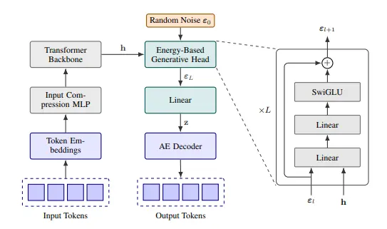
The underlying backbone of a CALM often remains the Transformer architecture—specifically, the decoder-only stack, similar to what powers GPT models. The core difference is found in the Output Head and the Training Objective.

Output Head: Modeling the Distribution

The final layer of a CALM's transformer doesn't project to the vocabulary size. Instead, it projects to a smaller set of values that define the parameters of the chosen continuous distribution. For example, if the model uses a simple Gaussian (Normal) distribution, the output head would predict:

1. The mean vector: A vector representing the predicted center point in the latent space for the next piece of content.
2. The covariance matrix: Which represents the uncertainty or spread around that predicted mean.

A more complex model might use a Mixture of Experts or a Mixture of Gaussians (MoG) head, predicting the means, covariances, and mixing coefficients for multiple distributions, allowing it to model a highly complex, multimodal distribution over the latent space.

Training Objectives: Density Estimation

The training objective moves away from the discrete Cross-Entropy Loss of LLMs. A CALM is trained to perform Negative Log-Likelihood (NLL) maximization with respect to the latent representation.

5. Comparison with Large Language Models (LLMs)

6. Inference and Generation Process

The generation process for a CALM is significantly more complex than the simple ArgMax or Top-P sampling in LLMs because the output is a point in space, not a token ID.

1. Prediction: The CALM processes the past sequence and outputs the parameters (Mean and Variance) of the continuous distribution for the next step.
2. Sampling: A latent embedding vector is sampled from this predicted distribution. This is the continuous output of the model.
3. Quantization/Mapping: The sampled continuous vector is not directly usable as a token. It must be mapped back to the discrete domain. This step usually involves a separate component, often a Vector Quantized (VQ) module or a simple Nearest Neighbor (NN) search against the dictionary of known token embeddings. The sampled vector is compared to all available token embeddings, and the one closest in Euclidean or Cosine distance is selected as the next discrete token.

This extra Quantization step adds computational overhead and introduces a potential source of error, sometimes called "quantization noise," which can lead to generated text or data that seems slightly 'off' or repetitive if the latent space isn't perfectly aligned with the discrete embeddings.

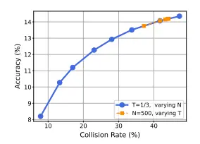
7. Experimental Results and Performance Evaluation

Evaluating CALMs is often done on generative tasks where the subtleties of the output matter. Benchmarks typically include:

• Perplexity (PPL): While still used, PPL on CALMs can be slightly misleading because the model is minimizing NLL on the embedding space, not the discrete tokens directly. A lower embedding NLL doesn't always translate perfectly to better human-rated text.
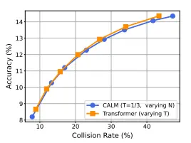
• Ablation Studies on Quantization: Researchers often test different quantization methods (e.g., VQ-VAE derived codes vs. simple k-NN) to see which best preserves the high-quality signals generated in the continuous space.
• Multi-Modal Tasks: CALMs have shown particular strength in mixed-modality generation, such as VQ-VAE based video or audio generation, where the continuous modeling of features like pixel intensity or mel-spectrogram coefficients provides smoother, more coherent outputs than discrete token models. For instance, in speech synthesis, continuous modeling of acoustic features leads to a much more natural and less 'stuttery' voice.

The current consensus is that for pure text generation, a discrete LLM remains the simplest and most performant architecture due to its direct objective. However, for tasks involving high-fidelity generation in a dense, continuous domain (like images, video, or high-quality audio), CALMs are often superior.

8. Applications and Use Cases

The ability of CALMs to model a continuous latent space opens up several unique and powerful applications:

• High-Fidelity Media Synthesis: Generating smooth, high-resolution images or videos where modeling subtle shifts in pixel values is critical. Think of them as the generative core of advanced VQ-VAEs or diffusion models that operate on discrete latent codes.
• Neural Speech Synthesis (Text-to-Speech): Modeling the acoustic features (like mel-spectrograms) as a continuous sequence results in far more natural and human-like voices than models that treat speech as a sequence of discrete units.
• Code and Molecular Structure Generation: Generating intermediate representations that might not have a direct, discrete token mapping, allowing for the exploration of novel, "in-between" structures or code snippets.
• Controllable Generation: Since the model outputs a mean $\mu$, one can subtly shift this mean vector before sampling to "steer" the generation in a specific direction (e.g., slightly more positive sentiment) without changing the prompt, offering finer-grained control than token-based LLMs.

9. Challenges and Open Research Problems

CALMs are not without their hurdles, and overcoming these is an active area of research:

• The Quantization Bottleneck: The necessity of mapping the continuous output back to a discrete token is the single largest challenge. If the mapping is poor, the high-quality signal from the continuous space is lost, and the output reverts to the quality of a standard discrete model.
• Computational Cost of Mapping: The nearest neighbor search required for quantization against a large embedding dictionary can be computationally expensive, slowing down inference compared to a simple matrix multiplication and softmax in a standard LLM.
• Latent Space Collapse: Ensuring that the continuous latent space remains rich and doesn't "collapse" (where the model only utilizes a small, confined region of the space) is a continuous objective in model stability and training.

‍